Improving FOSS photogrammetric workflows for processing large image datasets

Abstract

Background

In the last decade Photogrammetry has shown to be a valid alternative to LiDAR techniques for the generation of dense point clouds in many applications. However, dealing with large image sets is computationally demanding. It requires high performance hardware and often long processing times that makes the photogrammetric point cloud generation not suitable for mapping purposes at regional and national scale. These limitations are partially overcome by commercial solutions, thanks to the use of expensive and dedicated hardware. Nonetheless, a Free and Open-Source Software (FOSS) photogrammetric solution able to cope with these limitations is still missing.

Methods

In this paper, the bottlenecks of the basic components of photogrammetric workflows -tie-points extraction, bundle block adjustment (BBA) and dense image matching- are tackled implementing FOSS solutions. We present distributed computing algorithms for the tie-points extraction and for the dense image matching. Moreover, we present two algorithms for decreasing the memory needs of the BBA. The various algorithms are deployed on different hardware systems including a computer cluster.

Results and conclusions

The usage of the algorithms presented allows to process large image sets reducing the computational time. This is demonstrated using two different datasets.

Background

The generation of dense point clouds has been traditionally performed using active sensors like laser scanners due to the easiness, speed and ability to quickly capture millions of points. In the last decade, Photogrammetry has been living a second life pushed by the recent developments in Computer Vision, providing very dense and accurate point clouds compared to LiDAR techniques. Image-based approaches have the advantage of being cheaper than active sensors and they can provide colour and range information just in one acquisition. Photogrammetry is therefore replacing range techniques in many applications (such as archaeology, geology, etc.) due to their reduced costs and the introduction of turnkey platforms such as unmanned aerial vehicles (UAVs) that makes possible the acquisition of large datasets.

The trend in the photogrammetric community is to adopt larger datasets, increasing the image overlaps and the extension of the surveyed area, and to increase the resolution of the model using larger image formats. Many commercial solutions (Autodesk 123D Catch [1], Agisoft PhotoScan [2], Pix4Dmapper [3], etc.) and Free and Open-Source Software (FOSS) solutions (MicMac [4], VisualSFM [5], Bundler [6], openMVG [7], SFMToolkit [8], MVE [9], Theia [10], structure-from-motion [11], etc.) have been developed in the last years showing good results in many applications. The results achieved by image matching techniques are so promising that some countries are studying the possibility to replace periodic LiDAR acquisitions with airborne photogrammetric acquisitions. However, most of the solutions concentrated on the generation of 3D models on relatively small areas, and solutions for point cloud generation at a regional or national level are still unluckily limited.

Only few commercial software solutions (such as Acute3D [12]) are able to process city-scale regions and they are usually coupled with expensive dedicated hardware to generate the final products in a reasonable amount of time. Other solutions have also been specifically tailored to deal with large city-scale images datasets [13–15]. These solutions deal with clustered image sets, i.e. the total number of images is very large but even if the images belong to the same ares, these researches bypass this problem clustering the images in groups (for example images of a specific monument). In these approaches the technical challenge is more focused on the processing of the different chunks (to obtain the models of the different objects/clusters) and in their merging in a unique model, rather than in the processing of the whole block in a unique step.

Considering FOSS, many tools are available to perform complete photogrammetric workflows. The current solutions mostly target at running in a single computer. However, for large image sets this is not enough as the available memory and CPU is usually too limited, the data is too large to fit in a single disk and the processing time is too long. Therefore an accepted FOSS solution to manage regions at regional and national scale has not been developed yet. In this sense, it is crucial to understand the basic components of photogrammetric workflows in order to identify a strategy to deal with large image sets.

In this paper, the bottlenecks in the basic components of photogrammetric workflows are identified when dealing with large image sets, and the algorithms to overcome these problems are described. The algorithms are implemented as FOSS tools. The FOSS photogrammetric tool MicMac has been adopted as starting point. The use of clusters has been foreseen as possible solution to distribute the jobs on many machines, making possible the processing of big datasets.

The paper is organized as follow: the theoretical background and the problem statement are discussed in “Theoretical background and problem statement” section. The general structure of the MicMac tool is presented in “Methods” section while the algorithms are discussed in “Tie-points reduction algorithms” section and Distributed computing section. “Implementation” section contains implementation details. Experiments of test datasets are reported in “Results and discussion” section while the conclusions and future developments are discussed in “Conclusions” section.

Theoretical background and problem statement

Photogrammetry is the science of extracting 3D information from a set of overlapping images. Each image is ideally modeled as a central projection according to the pinhole camera model [16]: the projection center, the image point and the corresponding point in the space lie on the same line. The projective lines are then used to retrieve the position of points in the 3D space, given their 2D position on two or more images. Vice-versa, the position of a point on the images can be determined from its 3D coordinates in the space.

There are three basic components in photogrammetric workflows as depicted in Fig. 1: image calibration and orientation, dense image matching and true-orthophoto generation.

Fig. 1

Basic steps of photogrammetric workflows and the corresponding output of each component

The position and the attitude (georeferencing) where each image was acquired are recovered in the image orientation, while the focal length, the principal point position or distortions are determined in the image calibration. The image calibration is usually embedded in the image orientation process, thanks to the self-calibration process [17]. The image orientation process can be then divided in tie-points extraction, pose initialization and the Bundle Block Adjustment (BBA). In the tie-points extraction the position of the same object points in different overlapping images is performed. The tie-points extraction is usually performed using automated algorithms like SIFT [18], SURF [19], etc. The algorithms of automated tie-points extraction are able to detect thousands of points for each stereopair. It means that, on large blocks, several millions of tie-points can be extracted. This process can be particularly time consuming if the number of images is high as the correspondences between all the overlapping images to be matched exponentially increases. All the extracted tie-points are used in the pose initialization to sequentially determine a rough position of the images and the tie-points in the space: this step is usually fast and not computationally critical as it process few images per time. However, the pose initialization result needs to be refined by the BBA several times during the orientation process in order to prevent the diverge of the process. In each BBA, the tie-points have to be uploaded in a unique block: the higher is the number of points that have to be uploaded, the larger will be the memory occupied by the process. As a matter of fact, the requested memory on a large block is normally too high to be managed by a user-grade computer and the increase of the necessary RAM is not always possible.

After the image orientation, the position among images is known and a sparse point cloud with the tie-points position in 3D can be obtained. The dense image matching step can be performed to automatically extract a very high number of correspondences between the (homologous) pixels in overlapping images. The output of the dense image matching step is a colored dense point cloud or a depth map, i.e. a Digital Surface Model (DSM).

The current implementations are able to match one point in the space for each image pixel. The density of the point cloud is usually higher than the one that can be achieved by LiDAR techniques (depending on the Ground Sampling Distance, GSD, of the images), but it has the inconvenient to be extremely expensive from a computational point of view. A twofold correspondence between DSM points and corresponding image pixels is therefore established: a pixel on the DSM can be also back-projected to determine its coordinates on each of the overlapping images. The DSM can be therefore used to generate the true-orthophoto. The orthophoto is an orthogonal representation of the scene where the projective deformation of the images are removed exploiting the information given by the DSM.

Photogrammetric workflows are nowadays automated processes and the human interaction is limited. The development of large format cameras [20] and the increase in the image overlaps has led to the increase in the amount of data captured on the same area. This has resulted in a wider computational request to process large image datasets. The possibility to parallelize the process on CPUs and GPUs has just partially solved this issue as some steps cannot be easily divided in different processes and the steps are often too time consuming to make the whole process affordable and timely.

In this paper the above mentioned components of the photogrammetric workflow are analysed and solutions to speed the processing up in the most critical steps is presented. On the one hand, as the BBA requires all the data simultaneously in memory, a smart tie-points reductions is proposed to deal with large image sets. On the other hand, the tie-points extraction and the dense image matching the processing can be easily enhanced by using distributed computing (clusters or clouds). The reason is that the processes involved can be easily split in independent chunks. Each combination of stereopairs can be therefore distributed on independent processes for the tie-points extraction. In the same way, the scene is divided in small tiles and the dense image matching process can be independently processed on each of them. The true-orthophoto generation is usually performed together with the dense image matching. Thus, it can benefit from the same distributed computing solution used for the dense image matching. In the following section we will discuss the proposed solutions.

Methods

MicMac [4, 21–23] is a FOSS tool that executes photogrammetric workflows. It is highly configurable and allows to create and run different workflows tailored for different applications. After the images have been acquired, the steps to generate a dense point cloud and a true-orthophoto with MicMac usually include: executing the Tapioca command for the tie-points extraction, running the Tapas and the GCPBascule (or Campari) commands to perform the BBA and to georeference the image block, executing the Malt command for the dense image matching, running the Tawny command to generate the true-orthophoto and executing Nuage2Ply to convert the DSM and the true-orthophoto to the colored dense point cloud. Note that in the adopted MicMac pipeline is first necessary to create the true-orthophoto before the colored dense point cloud.

The solutions proposed in this paper have been developed starting from the the steps described above and using the data structures and exchange formats used in MicMac. The implemented algorithms are therefore additional or alternative steps that have been inserted in the workflow.

Tie-points reduction algorithms

The memory requirements for the BBA are in some cases simply unaffordable for large datasets. We propose an elegant solution that consists of running a tie-points reduction before the BBA. The tie-points reduction decreases the number of tie-points effectively decreasing the memory requirements of the BBA. The general idea is that a sufficient number of well distributed tie points in the overlapping images is sufficient to assure a stable and reliable image orientation, as it was commonly done in the traditional analogue Photogrammetry. Two different algorithms of tie-points reduction have been developed. A similar idea of tie-points reduction has been already introduced in a study conducted by Mayer [24]. However, in that case the tie-points reduction was part of the BBA. On the other hand, the proposed solutions are intended as a preliminary step to run before the BBA. In this way, the memory requirements of the BBA are decreased since the beginning preventing the need for large memory use.

In the following subsections the overview of the two different algorithms is given. The first algorithm performs the reduction using only the information provided by the tie-points in image space, while the second approach exploits the information provided by the tie-points both in image and object space to assure a better distribution in both spaces.

For an extended description and a study on the impact in the quality of the produced point cloud using the reduced set of tie-points, the reader can refer to the online report of the project “Improving Open-Source Photogrammetric Workflows for Processing Big Datasets” funded by the Netherlands eScience Center [25].

Tie-points reduction in the image space (RedTieP)

The input of the RedTieP algorithm consists of the set of images and their corresponding sets of tie-points. The relative position between overlapping images can be given as optional input to improve the process. The tie-points reduction is divided in tasks as depicted in Fig. 2, and there are as many tasks as images. The steps performed for each task can be described as follows:

• The master image, driving the reduction process, is initially determined: the ith task uses as master image the ith image from the list of images.

  Fig. 2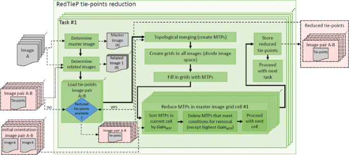

  

  Overview of the steps performed by the RedTieP algorithm

• The overlapping (related) images are selected considering the ones that share tie-points with the master image. A minimum number of common tie-points must be available to consider an image as related (10 points is the default value).

• The tie-points of all the related images are loaded. If the related image was a master in a previous task, then the reduced list of tie-points obtained by this earlier process is considered for that image.

• The loaded tie-points are topologically merged into multi-tie-points (MTPs). This means that a correspondence is created for the tie-points in different images pairs that relate to the same object point. A MTP keeps track of the number of image pairs in which a related tie-point is visible. This value is called multiplicity.

• The image space is divided in a regular grid (i.e. Von Gruber regions [26]). The algorithm fills the grids in with the positions of the MTPs. To locate a MTP in the image, the algorithm uses the position of the related tie-point in that image.

• The reduction is driven by the master image grid. Ideally the algorithm stores a single MTP (the related tie-points in fact) for each grid cell of the master image. However, some checks are done in order to guarantee that the distribution of tie-points in the related images is not damaged. For each grid cell of the master image, the MTPs are sorted according to their G a i n _MTP value given by formula 1.

  $$ Gain_{MTP} = \frac{M_{MTP}}{1 + (K \cdot \frac{A_{MTP}}{A_{median}})^{2}} $$

  (1)

  where M _MTP is the multiplicity of the MTP; K is a threshold value defined by the user (the default value is set equal to 0.5 from the performed tests); A _MTP is the estimated accuracy value of the MTP on the master image and it is computed as the highest residual value achieved by this point in the relative orientation with the other images; and A _median is the median of relative orientation residuals. Note that if K is zero or the relative orientation is not used, the G a i n _MTP is directly equal to the multiplicity of the MTP.

  The MTP with the highest G a i n _MTP in each grid cell of the master image is stored and the rest are removed if they meet the following conditions. A MTP can be removed (a) if none of its homologous points in the other images are part of the minimal set of reduced tie-points computed in a previous task with another master image (otherwise it would have been deleted before) and (b) if for all the image pairs another point is present in the same cell of the master image and in the corresponding cells of the overlapping images (in order to assure an homogeneous distribution of the points).

To overcome the cross-dependency of image pairs, the parallel algorithm guarantees that all the tasks running in parallel, at any time, process different image pairs. Noodles [27], a programmable workflow engine implemented in Python, has been adopted for the execution of these tasks in parallel.

Tie-points reduction in image and object space (OriRedTieP)

The second tie-points reduction algorithm is called OriRedTieP. It exploits the initial image orientation between adjacent stereo-pairs. In addition to the images and the tie-points per image pairs, this algorithm also requires the initial image orientation given by the pose initialization approach.

Figure 3 shows an overview of the steps performed by the OriRedTieP algorithm. From the initial pose estimation of the images, the algorithm projects the images in the 3D space to obtain the approximated 2D footprints. The object space is roughly defined by intersecting the tie-points extracted in the previous phase. The algorithm computes a bounding box containing the footprints of all the images and splits the bounding box in tiles. For each tile, the algorithm determines which images overlap it. The following of the process is split in tasks and the tiles are processed independently. For each tile, the algorithm follows a sequence of steps:

• The image pairs insisting on the tile and the corresponding tie-points are initially loaded. The tie-points with the estimated XY coordinates outside the tile are discarded.

  Fig. 3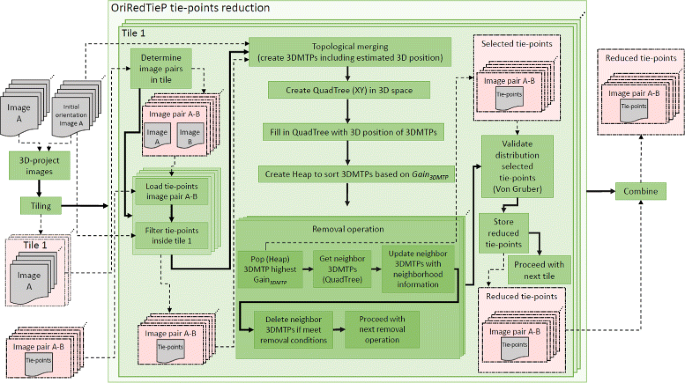

  

  Overview of the steps performed by the OriRedTieP algorithm

• The loaded tie-points are topologically merged into 3D multi-tie-points (3DMTPs). This means that a correspondence is created for the tie-points in different images pairs that relate to the same point in the object space. For each 3DMTP the algorithm determines its multiplicity (number of image pairs in which a related tie-point is visible) and its estimated 3D position in the space computed from the initial image orientation.

• A Quad-Tree with the 2D (XY) coordinates of the 3DMTPs is created.

• A Heap data structure is then generated to sort the 3DMTPs according to their G a i n _{3D M T P} value. The formula 2 is used to compute the G a i n _{3D M T P} .

  $$ Gain_{3DMTP} = \frac{M_{3DMTP}}{1 + \left(K \cdot \frac{E_{3DMTP}}{E_{median}}\right)^{2}} \cdot \left(0.5 + \frac{n_{3DMTP}}{N_{3DMTP}} \right) $$

  (2)

  where M _{3D M T P} is the multiplicity of the 3DMTP; K is a threshold value configurable by the user (the default value is 0.5); E _{3D M T P} is the estimated error when computing the 3D position of the 3DMTP given by the forward intersection; E _median is the median of estimated residual of all the 3DMTPs; N _{3D M T P} is the number of images where the tie-point is visible; n _{3D M T P} is the number of images where there are no other points in the neighborhood that have been already selected by the reduction process. Note that the value of n _{3D M T P} is dynamic and it changes every time a neighbor 3DMTP is preserved in the reduction process.

• The 3DMTPs are reduced in an iterative process using the Heap data structure. The 3DMTPs with higher G a i n _{3D M T P} are selected to be kept while their neighboring 3DMTPs are deleted only if the homogenous distribution of tie-points in the 3D object space is not compromised. In other words, a 3DMTP is usually deleted if it is visible in the same images of another 3DMTP that has been already preserved in the reduction process.

• Before storing the reduced set of tie-points, a final validation of the points in the image space is performed. This process is based on the von Gruber point locations [26]. For each deleted tie-point and in each image pair, the algorithm checks which is the closest tie-point which has been preserved. If that tie-point is further than a certain distance, then the deleted tie-point is re-added to the reduced list. The distance threshold is defined by the user.

The tasks for the different tiles can be executed in parallel. When all the tiles have been processed, the algorithm merges the tie-points of the image pairs that are processed in more than one tile.

Distributed computing

In the previous section we proposed two algorithms to tackle the memory requirements of the BBA when dealing with large image sets: the solution is to reduce the amount of processed data to a lower, but sufficient, number of tie-points. For the other challenging components of the photogrammetric workflows, i.e. tie-points extraction, dense image matching and true-orthophoto generation, distributed computing hardware systems can be used since the involved processes can be divided in chunks that can be processed independently (pleasingly parallel). In the next subsections we describe the distributed computing algorithms.

In “Methods” section we mentioned that in MicMac the true-orthophoto is actually generated before the dense colored point cloud. Therefore, both the dense image matching and the true-orthophoto generation are tackled by the distributed computing solution presented.

Tie-points extraction

The current single-machine implementation available in the Tapioca command of MicMac is the following:

• For each image of the dataset, the set of corresponding overlapping images is first determined. This process can be eased by the image geo-tag, reducing the number of homologous images to a small set. If the geo-tag is not available, then the whole dataset needs to be considered;

• For each image the features are extracted;

• For each stereopair, the features are matched to determine the candidate tie-points. The extraction and matching process are performed in parallel exploiting all the cores of the machine. However, this process is insufficient to process very large datasets.

The distributed computing solution is depicted in Fig. 4. The algorithm splits the list of stereopairs (image pairs) in chunks of N stereopairs where N is configured by the user: the first chunk contains the stereopairs from the position 0 to N-1 of the original list, the second chunk contains the stereopairs from the position N to 2N - 1 of the original list and so on. Each chunk can be processed independently and in a different machine. For each chunk, the algorithms works according to the following steps:

• The list of images in the chunk is determined from the list of image pairs. At this point the images are copied to the machine where the chunk is going to be processed.

  Fig. 4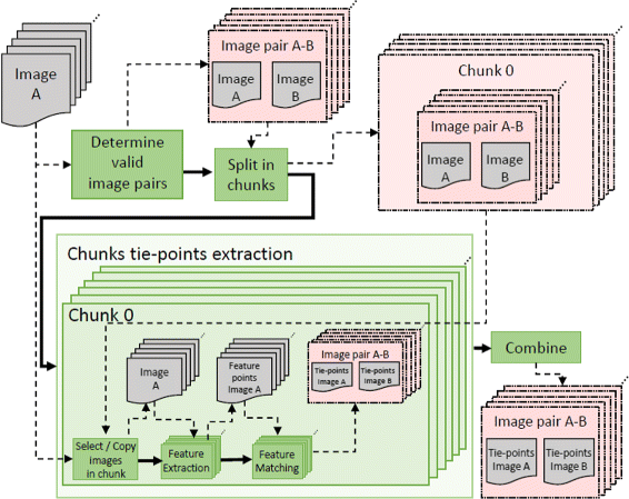

  

  Distributed computing implemented in the tie-points extraction

• The feature extraction on the images belonging to the chunk is performed.

• The feature matching among the image pairs of the chunk is computed.

The tie-points generated by all the chunks are finally combined. Note that since the distribution of the images in chunks is performed by image pairs, it may happen that different chunks use the same images. This means that the feature extraction step is duplicated in those images. This could be avoided by a two-step distributing computing solution where the feature extraction is completely performed in the first step while the second step is devoted to the feature matching among image pairs. However, due to implementation details (separating feature extraction and feature matching in Tapioca is not trivial) the two-step distributed computing solutions for tie-points extraction have not been considered at this stage of the work.

Dense image matching

The current single-machine implementation available in MicMac to generate the dense colored point cloud is the following: (i) the dense image matching is run and a dense depth map, i.e. a Digital Surface Model (DSM), is initially generated; (ii) using the DSM and the image spectral information, a true-orthophoto is then produced; (iii) the true-orthophoto and the DSM are finally used to generate the colored dense point cloud.

The process is generally divided in tiles and each of them is processed independently by a core. The GPU can be also adopted for this parallel process. However, the process can take very long times on a single machine. For a large dataset, a distributed computing solution is therefore required.

The distributed computing dense image matching algorithm is shown in Fig. 5. This algorithm has been specifically conceived for aerial images oriented in a cartographic reference system. The algorithm assumes that the Z component of the reference system does not have a real impact on the definition of the matching area. A 2D (XY) bounding box of the camera positions on the ground is therefore computed using the image orientation parameters. Then, this ground bounding box is split in tiles as shown in Fig. 6.

Fig. 5

Distributed computing implemented in the dense image matching

Fig. 6

Tiling procedure of the ground bounding box

Considering the 2D (XY) coordinates of the image projection centres, the algorithm determines the images that overlap each tile: these images are initially considered for this tile. Then the images partially overlapping with the tile are added as well: for this purpose, the images neighbouring the center and the vertices of the tile are considered. For each of these points the algorithm determines the n closest images (with n equals to 6, by default) and it adds them to the list of images, as shown in Fig. 7.

Fig. 7

Image selection strategy performed in each tile

After the list of overlapping images is determined for each tile, every independent process can be run in a different machine. For each tile the following tasks are executed:

• All the images corresponding to the processed tile as well as their orientation are copied to the machine where the tile is processed.

• The dense image matching algorithm is run considering the tile extension as area of interest. A DSM is therefore generated.

• The true-orthophoto of the tile is then generated.

• Using the DSM and the colour information of the true-orthophoto, the point cloud is generated.

• This point cloud is exported in order to be merged with the other tiles.

Since all the generated point clouds are in the same reference system they can be easily merged together.

Implementation

The tie-points reduction algorithms are implemented as stand-alone commands within the MicMac tool. The names of the commands are RedTieP and OriRedTieP.

The distributed computing algorithms for tie-points extraction and dense image matching are implemented in pymicmac (https://github.com/ImproPhoto/pymicmac). Pymicmac is a Python interface for MicMac workflows execution. It allows to define through a XML file photogrammetric workflows to be executed with MicMac. A sequence of MicMac commands is specified in the XML file. During the execution of each command pymicmac also monitors the usage of CPU, memory and disk. Pymicmac can also define parallel commands via XML, using a set of commands to be executed in parallel. This is what is used for the distributed computing tie-points extraction and the distributed computing dense image matching. The sequential and parallel commands defined in pymicmac can be executed with pycoeman (https://github.com/NLeSC/pycoeman), a Python toolkit for executing command-line commands. Pycoeman has tools to run both sequential and parallel commands locally (in the local computer) as well as parallel commands in a set of remote hosts accessible via SSH as well as in SGE clusters (computer clusters with Sun Grid Engine batch-queuing system).

Results and discussion

A set of experiments has been executed using the datasets reported in Table 1.

Table 1 Datasets used for the experiments

The two datasets have been specifically chosen to assess the performances of the tie-points reduction and the distributed computing. The first datased was acquired by an Unmanned Aerial Vehicle over a urban area in Gronau (Germany). The image overlap is quite irregular with 3 cm GSD. This dataset was chosen to assess the effectiveness of the tie-point reduction with highly overlapping and convergent image configurations. The second dataset is part of the acquisition yearly performed by the Waterschapshuis in The Netherlands: the image overlap is 60% alongtrack and 30% acrosstrack with 10 cm GSD. The number and size of the images prevent their processing on a single machine and it therefore represents a challenging dataset for the distributed computing task.

Tie-points extraction

The Gronau dataset has been used considering two different configurations: (i) the single-machine processing and (ii) the cluster processing. In both cases the feature extraction process has been supported by the geo-tag information. In the first case, this operation was executed with MicMac, i.e. using Tapioca, in a Ubuntu 14.04 Virtual Machine (VM) with 4 cores. Tapioca took 292,318.26 seconds, used all the available cores, and the average used memory was 13% out of the available 13.4 GB. Figure 8 (left) depicts the CPU and memory usage of Tapioca.

Fig. 8

CPU and memory usage for Tapioca execution in the single-machine (left) and in the DAS 4 cluster (right). The CPU usage ranges between 0 and 100% for each core (e.g. 4 × 100 = 400 is the maximum value for the single-machine solution)

In the distributed computing solution, the DAS 4 cluster [28] in TU Delft was used. The cluster has 32 nodes (only 23 are currently usable), and each node has 16 hyper-threaded cores at 2.4 GHz (512 hyper-threaded cores in total, only 368 can be currently used) and 24 GB RAM (768 GB in total, only 552 GB can be currently used).

A XML file with the set of commands was created in order to execute the distributed computing tie-points extraction in parallel. Each command processes a chunk of image pairs. The processing took 22,071.90 seconds, and in average 204 cores (out of the 512) and 13% of the RAM were used (97 GB out of the 768 GB). Figure 8 (right) depicts the CPU and memory usage of Tapioca in the DAS cluster.

Tapioca processes an image per time on each core of the PC and the RAM usage in both the tests is similar as the process is executed in the same way on a single machine or on each node of the cluster. On the other hand, the cluster processing reduces the computational time by a factor 10: this is less than expected considering the number of cores involved in the process. This can explained considering the communication times in the cluster (i.e. copy of files in remote) and the duplication of part of the processing as already explained in “Tie-points extraction” section.

Tie-points reduction and image orientation

The online report [25] of the project “Improving Open-Source Photogrammetric Workflows for Processing Big Datasets” contains a thorough study of the impact of a reduced set of tie-points in relation to the quality of the produced final point cloud. In that study various datasets and values for the options of the tie-points reduction commands were tested. In this paper, only some meaningful comparison are presented.

In particular, the comparison of the BBA results, i.e. Tapas in MicMac, using all the tie-points or a reduced set of tie-points are considered. The two commands RedTieP and OriRedTieP are tested. As in the previous section, the Gronau dataset has been used. In order to assess the quality of the orientations, the BBA residuals have been measured on the tie-points re-projection, on Ground Control Points (GCPs) and Check Points (CPs). The GCPs have been distributed using an uneven and very sparse distribution in order to better assess the possible deformations on the CPs due to the reduction of the used tie-points. Additionally, the number of iterations to converge the process has been recorded as well. The MicMac command GCPBascule is used to absolutely orient the images in the reference system and measure the residuals on the GCPs and CPs. GCPBascule performs a simple 7-parameter transformation where the parameters are estimated in a least square approach. This tool was preferred to Campari (traditional BBA, with GCP embedded in the process) because it does not introduce any non-linear effect in the model built by the photogrammetric data (i.e. the output of Tapas) and it allows a more frank estimate of the goodness of the photogrammetric models.

In Table 2 the comparison of three different cases is shown: the full set of tie points (No reduction), and the results achieved by the two reduction algorithms decreasing the full set of points to approximately the 5% of the original size. The Tapas residuals are only slightly degraded while the GCPs and CPs errors slightly increase when using the reduction algorithms. Both the algorithms show pretty similar results and their difference from the original implementation is not very relevant. By using the reduced set of tie-points Tapas is around thirty time faster, its memory usage decreases of about 90% and it requires much less iterations to converge to the solution. RedTieP is around five times faster than OriRedTieP because of the latter requires an initial image orientation given by the pose initialization while RedTieP only requires the image orientations between image pairs that are faster to compute.

Table 2 Comparison of executions of Tapas and GCPBascule when using all the tie-points or when using reduced sets by both tie-points reduction commands

Dense image matching

The Zwolle dataset has been used for the dense image matching test. This dataset is so large that its processing on a the single-machine solution (via MicMac commands Malt, Tawny and Nuage2Ply) would not be feasible because of the limited storage and the too long computational time. For this reason it was opted to run the process directly on the distributed solution in the DAS 4 cluster generating a point cloud with 25% of the maximum density achievable (i.e. 1 point every 4 pixels, 20 cm avarage spacing between points) in order to fulfill the 15-minutes-per-job policy of the cluster: the whole process was divided in 3,600 tiles. The execution took 65,350 seconds, and in average 70 cores were used (out of 512) and only 2% RAM was used (15 GB of the 768 GB) due to the very little dimensions of each tile. In Fig. 9 the CPU and memory usage of the distributed computing dense image matching in DAS 4 are reported.

Fig. 9

CPU and Memory usage for the distributed computing dense image matching execution in the DAS 4 cluster. The CPU usage ranges between 0 an 100 for each core of the cluster: 70 cores were used on average

The final point cloud had 15 billion points and an average density of 25 points per square meter. The full resolution would have required 4 times more tiles and longer computational time. In that case an estimated density of 100 points per square meter would have been reached. For the visualization of the final point clouds we used Potree [29, 30] and the Massive-PotreeConverter [31]. Snapshots of the visualization are shown in Figs. 10 and 11. The images were acquired with low overlaps (60% along-track, 30% across-track), as the flight was not conceived to generate a dense point cloud. For this reason, the quality of the point cloud is quite low, with several regions affected by noise and not accurate 3D reconstructions. However, the quality of the point clouds was out of the scope of this work as this contribution was a proof-of-concept for the processing of large datasets. The color equalization among different tiles was still a problem as the true-orthophotos used to color the point cloud was equalized independently and in a different way on each tile.

Fig. 10

Snapshot of the point cloud generated by the distributed computing dense image matching. The different tiles are visible due to a different color equalization per tile

Fig. 11

Zoom on a detail of the point cloud generated by the distributed computing dense image matching

Conclusions

An innovative approach devoted to the efficient and reliable photogrammetric processing of large datasets has been presented in this paper. The bottlenecks in the basic components of photogrammetric workflows when dealing with large datasets have been pointed out at first. For each of them an efficient solution has been conceived using the FOSS tool MicMac. The tie-points extraction and the dense image matching (point cloud generation) are similar problems. In these cases, the amount of data to be processed is very large and it cannot be reduced. The positive aspect is that the process can be parallelized and distributed on large clusters, as demonstrated in this paper. On the other hand, the BBA is not easily divisible and an algorithm to optimize the amount of processed data has been developed. The developed algorithms allow the processing on user-grade machines, preventing the need for more powerful devices on large datasets.

The achieved tests have provided encouraging outcomes in all the developed tools, showing that the developed algorithms decrease the computational time. This paper represents a proof of concept and many details will be improved in the future in order to further optimize the whole process. The tie-points reduction would greatly benefit from the division of the two tasks (feature extraction and feature matching), reducing the number of stereopairs that have to be matched in the cluster processing. The dense point cloud generation would need some improvement in the radiometric equalization of the point cloud color.

The Zwolle dataset was challenging due to the high number of (large format) images processed. However, higher image overlaps would have allowed better results using the same dense image matching algorithm. New tests on more challenging datasets will be performed to further validated the developed algorithms.